Xpansiv Data SDK and API Usage Guide

Overview

This guide demonstrates how to use the Xpansiv Data API to authenticate, download data, and generate insights through visualization. The workflow combines curl commands for API interactions with Python scripting for data analysis and visualization.

1. Obtaining Tokens

Before accessing the Xpansiv Data API, you need to authenticate and obtain access tokens.

Authentication Request:

curl -u 'username:Password' https://api.xsignals.xpansiv.com/auth/login

Response:

The command will return two tokens:

• Bearer Token - Used for API authorization in subsequent requests
• Refresh Token - Used to obtain new bearer tokens when they expire

Best Practice: Store the bearer token in an environment variable for secure and easy access throughout your session.

export NG_TOKEN="your_bearer_token_here"

2. Downloading Data

Once authenticated, you can query the data lake to identify and download files to your local machine.

Searching for Files

The following example searches for files in the placeholder group name "Example Contracts_RECs" and retrieves up to 100 results:

curl \
  -H "Authorization: Bearer $NG_TOKEN" \
  'https://api.xsignals.xpansiv.com/file/search?size=100&query=groupName%Example%20Contracts_RECs' \
  | jq -r '.items[] | "\(.fid),\(.fileName)"' \
  | while IFS=',' read -r file_id file_name; do
      # Creates a unique file name using the file ID to prevent overwriting
      local_file_name="${file_name%.csv}_${file_id}.csv"
      
      echo "Downloading $file_name (ID: $file_id) to $local_file_name..."
      
      curl \
        -H "Authorization: Bearer $NG_TOKEN" \
        "https://api.xsignals.xpansiv.com/file/$file_id/download" \
        > "$local_file_name"
    done

What This Does:

1. Queries the API - Searches for files in the specified group
2. Parses Results - Uses jq to extract file IDs and names from the JSON response
3. Downloads Files - Iterates through each file and downloads it with a unique name based on the file ID
4. Prevents Overwriting - Appends the file ID to each filename to ensure uniqueness

Environment Variable: The $NG_TOKEN variable contains your bearer token for authorization.

3. Confirming Files Are Ready

After downloading, verify that the data has been successfully imported to your local machine.

ls -lh *_*.csv
head -n 5 your_downloaded_file.csv

Take a quick glance at the files to ensure they were imported properly and aren't corrupted.

4. Drawing Value From Data

Data Filtering

Use Python scripting to filter and prepare your data for analysis. The following example filters based on specific columns:

# Filter data based on PeriodRel and Symbol columns
fdf = df[(df['PeriodRel'].isin(sel_per)) & (df['Symbol'].isin(sel_cont))].copy()

Key Columns:

• PeriodRel - Period relationship/term for the contract
• Symbol - Identifier for the specific asset or contract

You can filter on these columns or others based on your analytical needs. For more information on column terminology specific to Xpansiv Data workflows, please refer to the Data Dictionary section.

Plotting Price With Dates

A significant benefit of the Xpansiv Data system is the ease of accessing and storing data in time series formats. This makes downstream applications like plotting prices against time much simpler.

# Plot data for each contract symbol
for cont in sel_cont:
    group = fdf[fdf['Symbol'] == cont]
    # Add trace using group['Date'] and group['Mid'] or group['Mid_MA']
    # ... plotting code here

What This Does:

• Iterates through selected contract symbols
• Filters data for each contract
• Plots price data (such as Mid prices or moving averages Mid_MA ) against dates

Data Points:

• Mid - Mid-price reflecting the average price for assets
• Mid_MA - Moving average of mid-prices
• Date - Timestamp for each data point

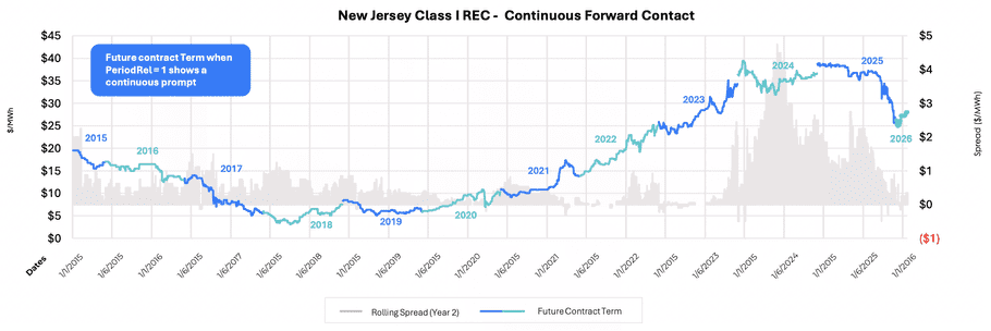
5. Example: Market Insight Visualization

Let's visualize price trends for a specific product and term range.

Scenario: Filter on the product "New Jersey Class 1 REC" for terms 2026 to 2030, then plot contract prices over time.

import streamlit as st
import pandas as pd
import plotly.express as px

# Load downloaded data
df = pd.read_csv('your_downloaded_file.csv')

# Filter for specific product and terms
sel_per = [2026, 2027, 2028, 2029, 2030]
sel_cont = ['NJ_Class1_REC']

fdf = df[(df['PeriodRel'].isin(sel_per)) & (df['Symbol'].isin(sel_cont))].copy()

# Create visualization
fig = px.line(fdf, x='Date', y='Mid', color='Symbol', title='Contract Prices Over Time')
st.plotly_chart(fig)

Visualization Tools:

This example uses Streamlit, but you can achieve similar results with:

• Seaborn - Statistical data visualization
• Plotly - Interactive plotting library
• Matplotlib - Basic plotting capabilities

Visualizing price of assets over time using API

Key Benefits

Speed and Scalability: A combination of basic curl commands and simple scripting provides:

• Fast access to market insights
• Scalability to accommodate future data inputs
• Reproducible workflows for ongoing analysis

Time Series Advantages:

• Native time series format simplifies temporal analysis
• Easy plotting of prices against time
• Support for trend analysis and forecasting

API Reference Summary

Authentication Endpoint

POST https://api.xsignals.xpansiv.com/auth/login

File Search Endpoint

GET https://api.xsignals.xpansiv.com/file/search?size=<size>&query=<query>

File Download Endpoint

GET https://api.xsignals.xpansiv.com/file/<file_id>/download

Best Practices

1. Token Security - Always store bearer tokens in environment variables
2. File Naming - Use unique identifiers (like file IDs) to prevent overwriting
3. Data Validation - Verify downloaded files before processing
4. Error Handling - Implement proper error handling in production scripts
5. Documentation - Refer to the Data Dictionary for column definitions and terminology

Next Steps

• Explore additional filtering options based on your data columns
• Implement automated data refresh workflows
• Build dashboards for real-time market monitoring
• Integrate with other data sources for comprehensive analysis